We Live in Interesting Times.
The Stock Market’s Response to Changes in Commercial Banks’ Reserves.
- Recent Experience.
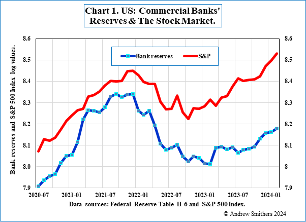
The US stock market has moved since mid-2020 with changes in the level of commercial banks’ reserves with the Federal Reserve, as Chart 1 shows. This could be a case of data mining (aka data dredging1), but this is unlikely because there is: (i) a straightforward explanation for the relationship, as set out in Section 2, and (ii) it is shown in Appendix 1 when all the data available are used – though to a less marked extent than over the past 4 years.
Three variables can be readily identified from the data which cause the US stock market to fluctuate around fair value. These are fluctuations in (i) profits per share, (ii) nominal bond yields, and (iii) household liquidity. The importance of these varies at different times. Bond yields dominate when there are sharp changes in nominal interest rates, as they did from 1960 to 2010, but were unimportant from 1940 to 1950, when companies were denied access to bond markets by wartime regulations, and from 1950 to 1960, when leverage was being rebuilt. Liquidity became the dominant variable with the introduction of QE in 2009 and again over the past four years as commercial banks’ reserves were first reduced by QT (Quantitative Tightening) and then boosted by massive and largely unfunded fiscal deficits. These changes are set out in Appendix 2.
- How Banks’ Reserves Affect the Stock Market.
Household financial assets consist primarily of cash, bonds, and equities. If households have the level of liquidity they desire, then their only decision is between bonds and equity. If they buy equities, they must sell bonds and, as companies seek to have a stable ratio of interest payments to profits (Appendix 3), corporate decisions tend to offset those of households.
As there is a time delay between fluctuations in household preferences and the offsetting behaviour of companies, changes in these preferences provide an unpredictable element of statistical noise to the level of share prices, but only if they wish to change their liquidity do households have a more than fleeting impact on the prices of shares and bonds. Changes in share prices, without any alteration in the level of liquidity, depend largely on fluctuating changes in corporate leverage in response to alterations in interest rates and profits.
Liquidity rises if the government runs a budget deficit not financed by the issue of bonds, or if the central bank buys bonds (QE). Commercial banks’ reserves then rise by the same amount as liquidity.
- Liquidity Does Not Vary with M2 or the Monetary Base.
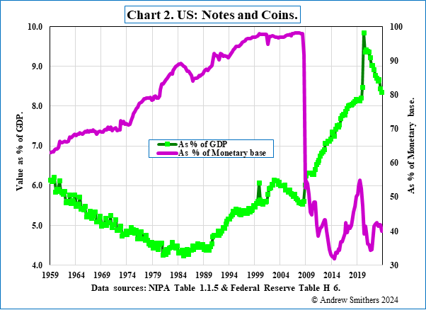
The monetary base consists of cash, in the form of notes and coins, whether they are held by banks, companies, households or criminals, plus the reserves of commercial banks held with central banks. Why the value of notes and coins in the economy should fluctuate is far from clear and they have, as Chart 2 shows, amounted to up to 92% of the monetary base. In the absence of any satisfactory explanation of why demand for them varies, references to the monetary base convey virtually no information and certainly none about liquidity.
M2 rises if, via the intermediation of banks, some households lend more to other households. The liquidity of the lenders then rises, and so does the illiquidity of the borrowers. There is no net change in liquidity as M2 rises and it does not therefore measure liquidity.
- Banks’ Reserves Affect the Economy Not Just the Stock Market.
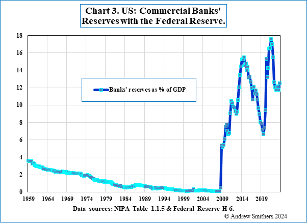
Banks’ reserves, for which the Federal Reserve publishes data from January 1959, have risen from 1% of GDP in 2009 to 12% today (Chart 3). They are currently rising (Chart 1) and, as the Federal Government in Q4 borrowed 10.3% of GDP2, this will continue at a rapid rate, unless there is a sharp reduction in the deficit or a large rise in interest rates so that the deficit can be funded by bond sales.
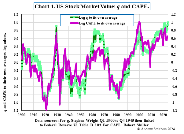
Profits are likely to decline if the fiscal deficit contracts, and liquidity will fall if funding policy changes. In either event the stock market is likely to weaken and there is a high risk of a sharp major decline given the current overvaluation of US equities illustrated in Chart 4.
The level of commercial banks’ reserves with the Federal Reserve deserves attention, not only as a measure of liquidity, with its consequent importance for the stock market, but because of its importance for the economy. Banks in the US, in common with other developed economies, can create money – the system known as fractional banking – but their ability to do so is limited by the level of their reserves. They must hold enough notes to allow depositors to withdraw funds, so, when their reserves are low, increased bank lending requires more reserves. When reserves are low central banks can readily control bank lending by limiting the expansion of reserves and thus the level of M2. This is more problematic when banks have ample reserves. The ease with which commercial banks can then expand their lending, raises the concern that growth in M2 can only be controlled by sharp changes in interest rates through large interventions in the bond market (open-market operations). When in 1936 the Federal Reserve sought to avoid the possible problem that large reserves might present by sterilizing them, the result was a major recession. “Motivated mainly by a desire to put the System in a position where it could use open—market operations to affect the economy in the future should it wish to do so …in 1936 and 1937 the Federal Reserve doubled reserve requirements.”3 This was followed by a jump in unemployment from 14.3% in May 1937 to 19.0% in June 1938 and manufacturing output fell by 37%.
- Can The Current Policy Continue?
As the yield curve is habitually upward sloping, it is expensive for governments to fund by issuing bonds rather than allowing bank reserves to expand. Nonetheless, governments have habitually sought to fund their debt. Either they have simply been foolish, or failing to fund must involve risk. Large reserves due to underfunding may render it difficult for central banks to control the level of M2/GDP without the sharp rises in interest rates which precipitate recessions; and monetarists may be correct in claiming that inflation follows if M2/GDP is not constrained.
.
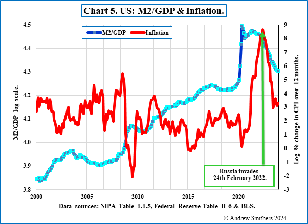
The importance of monetary aggregates is, to put it mildly, much disputed. The monetarist case has, however, been boosted by recent experience, as illustrated in Chart 4, which shows that inflation rose dramatically following a sharp rise in the ratio of M2/GDP and preceded Putins’s invasion of the Ukraine.
A halt to the expansion of bank reserves requires some combination of tighter fiscal or monetary policy, which seems unlikely, as any effective combination threatens to create a severe recession. The experience of 1936-1937 suggests that seeking to sterilize reserves by increasing reserve requirements also has high risks. So the current prospect is that commercial banks’ reserves will continue to grow and support asset prices. We do not know whether this is possible without either a resurgence of inflation or a stock market collapse – we are therefore witnessing an interesting and previously untested experiment with the US economy.
We, and economists in particular, have the dubious privilege of living in interesting times.
Appendix 1.
Correlation between S&P 500 and Commercial Banks’ Reserves.
The Federal Reserve publishes data on commercial banks’ reserves from 1st January 1959, with the most recent datum point being for February 2024.
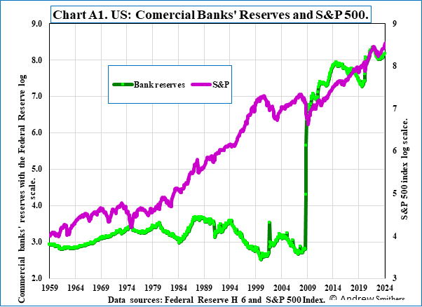
In Chart A1 I compare the level of these reserves with the level of the S&P 500 using a log scale for both, so that the proportionate changes are the same for both variables. Over this period they have had a positive correlation of 0.68539 (R2 0.46976). These data are consistent with the assumption that liquidity, as measured by banks’ reserves, is important for the market’s level, but is not the only determinant, and others can at times be of overwhelming importance.
Appendix 2.
Fluctuations in EPS, Bond Yields, Liquidity and Stock Market Value.
Companies borrow more when interest rates are low; except from 1940 to 1970. At other times non-financial companies have sought, in aggregate, to have their interest payments covered 5 times by profits, measured after depreciation and before interest and tax. From 1940 to 1950 companies were denied access to debt markets as priority was given to government borrowing. Corporate leverage therefore fell sharply, only to rise again once the restrictions ended. By 1970 corporate debt had recovered to its pre-war level.
If companies seek to maintain a stable level of interest cover, they will borrow more if profits rise or interest rates fall. When they borrow more, they use less equity and, if there are no other changes, this will push up share prices.
In the absence of changes in profits, interest rates or liquidity ratios, households can switch their portfolio between debt and equity. If they seek to own more debt and less equity, bond yields will fall and companies will respond by borrowing more debt and using less equity. As mentioned in Section 2, fluctuations in households’ portfolio preferences will thus be offset by companies.
It is only if liquidity, or the perceived need for it changes, that households will have more than an ephemeral impact on the stock market. If liquidity rises, households will seek to increase their ownership of equities and bonds and the prices of both will tend to rise.
The stock market will thus respond to changes in profits and interest rates because companies will vary their levels of equity issues, buybacks and dividends in response to those changes. Shareholders respond badly to new equity issues and dividend cuts and, as managements like to keep their jobs, changes in the level of buy-acks, which include reductions in equity from debt-financed takeovers, are the preferred method of adjustment.
It is nominal rather than real interest rates which determine changes in leverage. Although profits also respond to changes in inflation, they respond much more slowly than interest rates.
Swings in the stock market away from fair value have been driven by changes in nominal interest rates, EPS, profits, and liquidity. The importance of each variable has changed and the weight of their influence has fluctuated.
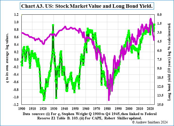
Chart A3 illustrates how market value responded negatively to the rise in the bond yield from 1963 to 1983 and then positively to its fall from 1983 to 2000, with the result that changes in bond yields had a highly significant impact on the market from 1963 to 2000.
Between 2000 and 2004 there was also, as Table A1 shows, a more limited relationship (R2 =0.26 vs 0.74 for 1963 to 2000).
| Table A1. US: Correlations between q and Long-dated Bond Yields 1900 to 2022. (Data sources: (i) For q, Stephen Wright Q1 2000 to Q4 1945 linked to Federal Reserve Table B 103. (ii) For CAPE, Robert Shiller.) | ||
| Coefficient of Correlation | R2 | |
| 1900 to 1963 | 0.148518 | 0.022058 |
| 1963 to 2000 | -0.86068 | 0.740773 |
| 2000 to 2024 | -0.5085 | 0.258574 |
| 1900 to 2024 | -0.26154 | 0.068402 |
| Table A2. Commercial banks’ reserves and q. (Data sources: Stephen Wright, Federal Reserve Z1 Table B. 103 &Table H 6 and NIPA Table 1.1.5.) | ||
| Coefficient of correlation | R2 | |
| Q1 1959 to Q1 2009 | -0.371444491 | 0.13797101 |
| Q1 2009 to Q4 2016 | 0.913815716 | 0.835059164 |
| Q1 2017 to Q3 2018 | -0.854728706 | 0.730561161 |
| Q4 2018 to Q4 2023 | 0.612625999 | 0.375310614 |
| Q1 1959 to Q4 2024 | 0.440441322 | 0.193988558 |
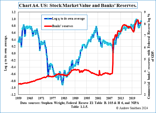
Chart A4 and Table A2 show a similar patten with regard to liquidity. From 1959 to 2009, when banks’ reserves varied little relative to GDP, there was no relationship between liquidity and market value.
In the absence of long-term profit data for quoted companies I assume that changes in profits rather than in share numbers have dominated changes in EPS and compare those with changes in q. Using all available data the correlations are low but, as Table A3 illustrates, they are stronger when measured over two years than for shorter or longer periods and this is therefore the measurement period used in Chart A5.
| Table 3. Coefficients of correlation between log changes in q and EPS Q1 1900 to Q2 2023. (Data sources: Stephen Wright, Federal Reserve Z1 Table B. 103 & Robert Shiller). | ||||||||
| Period | 1Q | 2Q | 1 year | 2 years | 3 years | 4 years | 5 years | 10 years |
| Coefficient | 0.07 | 0.11 | 0.15 | 0.23 | 0.22 | 0.20 | 0.20 | 0.07 |
.
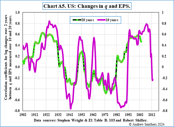
Chart A5 shows the correlation coefficients for log changes in q and EPS measured over 10 and 20 years. Except for 1982 to 1992, the two series show a similar pattern, while the volatility of this series measured over 5 years is too marked to provide helpful information.4 Assuming that profit changes are always important for the stock market, periods of negative correlation will be those when changes in other variables dominate other causes for fluctuations in the market’s value. These are, as shown in Chart A5, 1940 to 1950, when the stock market was depressed by companies’ lack of access to debt markets due to wartime regulations, and 1960 to 1983, when it was depressed by the rapid rise in the cost of debt. The sharp drop in the correlation shown by the 10 year data since 2008 is consistent with the assumption that since then alterations in banks’ reserves have been the major determinant of changes in market value.
Appendix 3.
Savings and Liquidity Preference.
I use a model in which the household sector is assumed to save for two purposes, which are: (i) precautionary, which need to be held in cash so that full value can be realised in the short-term for holidays and emergencies, such as illness and unemployment, and (ii) retirement, for which bonds and equities with their higher returns are appropriate.
The need for precautionary savings will vary for individuals if there are changes in their risks of unemployment or ill health, but for the population overall this is likely to be stable, other than in times of crisis. In their absence, changes in commercial banks’ reserves will therefore measure changes in liquidity relative to households’ perceived need for liquidity, subject to the proviso that over the long term changes in health insurance and the perceived risks of unemployment can alter the need for precautionary savings for the population overall.
1 As preferred in The Art of Statistics (2019) by David Spiegelhalter Pelikan Books,
2 Z1 Table D2 as % of NIPA 1.1.5.
3 Does Monetary Policy Matter? A New Test in the Spirit of Freidman and Schwartz (1989) by Christina Romer and David Romer NBER Working Paper No. 2966.
4 The standard deviation when measured over 5 years is 0.56, over 10 years is 0.47 and over 20 years is 0.35.